
Pierre Gaillard, Yannig Goude

opera useful?opera is a R package that provides several algorithms to
perform robust online prediction of time series with the help of expert
advice. In this vignette, we provide an example of how to use the
package.
opera useful?Consider a sequence of real bounded observations y1, …, yn to be predicted step by step. Suppose that you have at your disposal a finite set of methods k = 1, …, K (henceforth referred to as experts) that provide you before each time step t = 1, …, n predictions xk, t of the next observation yt. You can form your prediction ŷt by using only the knowledge of the past observations y1, …, yt − 1 and past and current expert forecasts xk, 1, …, xk, t for k = 1, …, K. The package opera implements several algorithms of the online learning literature that form predictions ŷt by combining the expert forecasts according to their past performance. That is,
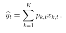
These algorithms come with finite time worst-case guarantees. The monograph of Cesa-Bianchi and Lugisi (2006) gives a complete introduction to the setting of prediction of arbitrary sequences with the help of expert advice.
The package opera provides three important functions:
mixture to build the algorithm object, predict
to make a prediction by using the algorithm, and oracle to
evaluate the performance of the experts and compare the performance of
the combining algorithm.
opera is now available on CRAN, so you can install it with:
install.packages("opera")You can also install the development version of opera with the package devtools:
install.packages("devtools")
devtools::install_github("dralliag/opera")
You may be asked to install additional necessary packages. You can install the package vignette by setting the option: build_vignettes = TRUE.
Here, we provide a concrete example on how to use the package. To do so, we consider an electricity forecasting data set that includes weekly observations of the French electric load together with several covariates: the temperature, calendar information, and industrial production indexes. The data set is provided by the French National Institute of Statistics and Economic Studies (Insee).
library(opera)
set.seed(1)First, we load the data and we cut it into two subsets: a training set used to build the experts (base forecasting methods) and a testing set (here the last two years) used to evaluate the performance and to run the combining algorithms.
data(electric_load)
attach(electric_load)
idx_data_test <- 620:nrow(electric_load)
data_train <- electric_load[-idx_data_test, ]
data_test <- electric_load[idx_data_test, ]
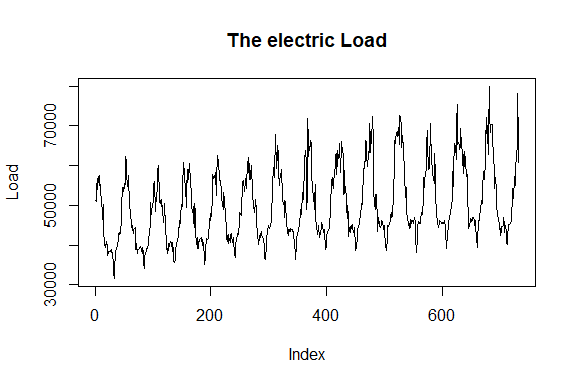
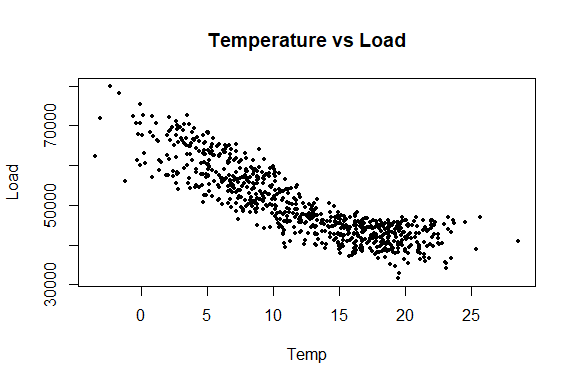
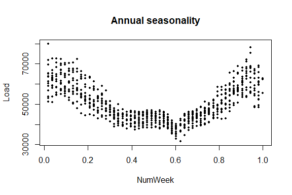
The data is displayed in the following figures.
plot(Load, type = "l", main = "The electric Load")
plot(Temp, Load, pch = 16, cex = 0.5, main = "Temperature vs Load")
plot(NumWeek, Load, pch = 16, cex = 0.5, main = "Annual seasonality")
Here, we build three base forecasting methods to be combined later.
mgcv
package:library(mgcv)
gam.fit <- gam(Load ~ s(IPI) + s(Temp) + s(Time, k=3) +
s(Load1) + as.factor(NumWeek), data = data_train)
gam.forecast <- predict(gam.fit, newdata = data_test)# medium term model
medium.fit <- gam(Load ~ s(Time,k=3) + s(NumWeek) + s(Temp) + s(IPI), data = data_train)
electric_load$Medium <- c(predict(medium.fit), predict(medium.fit, newdata = data_test))
electric_load$Residuals <- electric_load$Load - electric_load$Medium
# autoregressive correction
ar.forecast <- numeric(length(idx_data_test))
for (i in seq(idx_data_test)) {
ar.fit <- ar(electric_load$Residuals[1:(idx_data_test[i] - 1)])
ar.forecast[i] <- as.numeric(predict(ar.fit)$pred) + electric_load$Medium[idx_data_test[i]]
}caret packagelibrary(caret)
gbm.fit <- train(Load ~ IPI + IPI_CVS + Temp + Temp1 + Time + Load1 + NumWeek, data = data_train, method = "gbm")
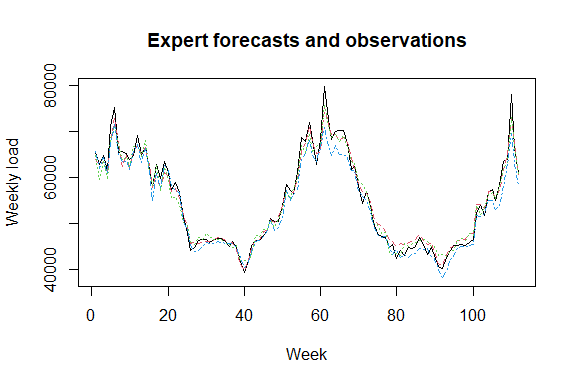
gbm.forecast <- predict(gbm.fit, newdata = data_test)Once the expert forecasts have been created (note that they can also be formed online), we build the matrix of expert and the time series to be predicted online
Y <- data_test$Load
X <- cbind(gam.forecast, ar.forecast, gbm.forecast)
matplot(cbind(Y, X), type = "l", col = 1:6, ylab = "Weekly load",
        xlab = "Week", main = "Expert forecasts and observations")
To evaluate the performance of the experts and see if the aggregation rules may perform well, you can look at the oracles (rules that are used only for analysis and cannot be design online).
oracle.convex <- oracle(Y = Y, experts = X, loss.type = "square", model = "convex")
print(oracle.convex)
plot(oracle.convex)
#> Call:
#> oracle.default(Y = Y, experts = X, model = "convex", loss.type = "square")
#>
#> Coefficients:
#>    gam    ar    gbm
#>  0.719 0.201 0.0799
#>
#>                       rmse   mape
#> Best expert oracle:   1480 0.0202
#> Uniform combination:  1560 0.0198
#> Best convex oracle:   1440 0.0193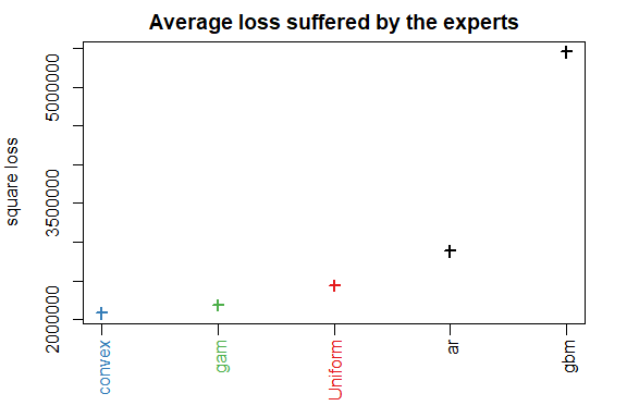
The parameter loss.type defines the evaluation
criterion. It can be either the square loss, the percentage loss, the
absolute loss, or the pinball loss to perform quantile regression.
The parameter model defines the oracle to be calculated.
Here, we computed the best fixed convex combination of expert (i.e.,
with non-negative weights that sum to one).
The first step consists in initializing the algorithm by defining the type of algorithm (Ridge regression, exponentially weighted average forecaster,…), the possible parameters, and the evaluation criterion. If no parameter is defined by the user, all parameters will be calibrated online by the algorithm. Bellow, we define the ML-Poly algorithm, evaluated by the square loss.
MLpol0 <- mixture(model = "MLpol", loss.type = "square")Then, you can perform online predictions by using the
predict method. At each time, step the aggregation rule
forms a new prediction and update the procedure.
MLpol <- MLpol0
for (i in 1:length(Y)) {
  MLpol <- predict(MLpol, newexperts = X[i, ], newY = Y[i])
}
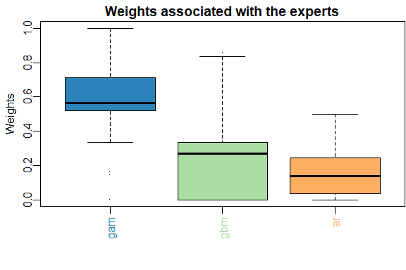
The results can be displayed with method summary and
plot.
summary(MLpol)
#> Aggregation rule: MLpol
#> Loss function:  squareloss
#> Gradient trick:  TRUE
#> Coefficients:
#>    gam    ar gbm
#>  0.577 0.423   0
#>
#> Number of experts:  3
#> Number of observations:  112
#> Dimension of the data:  1
#>
#>         rmse   mape
#> MLpol   1460 0.0192
#> Uniform 1560 0.0198plot(MLpol)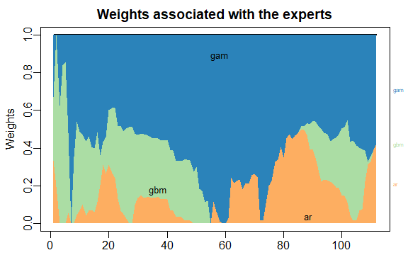
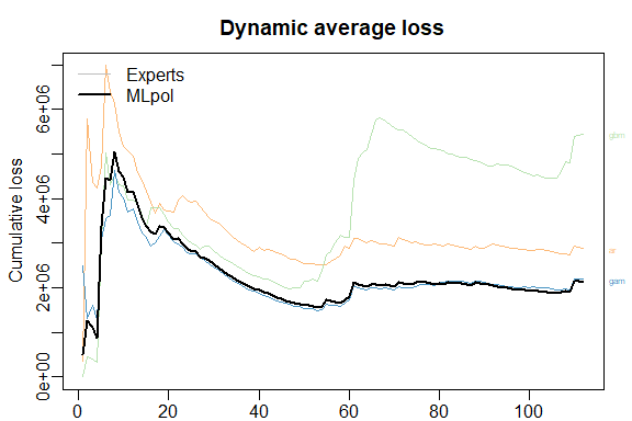
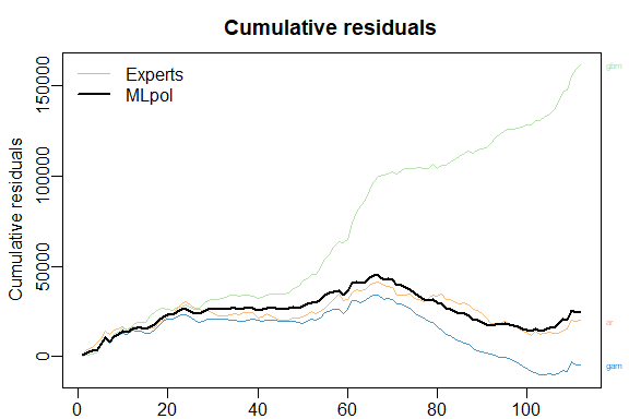
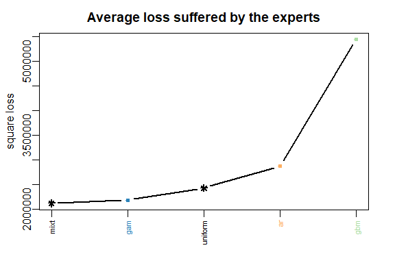
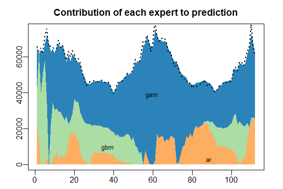
The same results can be obtained more directly:
predict specifying
online = TRUE to perform online prediction.MLpol <- predict(MLpol0, newexpert = X, newY = Y, online = TRUE)MLpol <- mixture(Y = Y, experts = X, model = "MLpol", loss.type = "square")The vector of predictions formed by the mixture can be obtained through the output prediction.
predictions <- MLpol$predictionNote that these predictions were obtained sequentially by the algorithm by updating the model coefficients after each data. It is worth to emphasize that each observation is used to get the prediction of the next observations but not itself (nor past observations).
In real-world situations, predictions should be produced without
having access to the observed outputs. There are several solutions to
get them with opera.
Using the predict method with the arguments *
online = FALSE: the model coefficients are not updated
during the prediction. * type = response: the predictions
are returned and not an updated model.
newexperts <- X[1:3, ] # Experts forecasts to predict 3 new points
pred <- predict(MLpol, newexperts = newexperts, online = FALSE, type = 'response')
#> [1] 64397.10 61317.41 63571.59The same result can be easily obtained by using the last model coefficients to perform the weighted average of the expert advice.
pred = newexperts %*% MLpol$coefficients#> [1] 64397.10 61317.41 63571.59In some situations, the aggregation model cannot be updated at each step due to an operational constraint. One must predict the time-series y1, …, yn block by block. For example, a weather website might want to make a daily forecast of the next day’s temperature at hourly intervals. This corresponds to block by block predictions of 24 observations.
Let’s say that in the above example, instead of making a weekly
prediction, we need to predict every four weeks, the consumption of the
next four weeks. Below we show two different ways to use the
opera package to do this.
Note that the outputs
y1, …, yn to be
predicted step by step can be d-dimensional in
opera. In this case, the argument Y provided
to the function mixture should be a matrix, where each line
corresponds to the output observed at time t; the argument
experts must be an array of dimension
T × d × K such that
experts[t,:,k] is the prediction made by expert k
at iteration t. These predictions of dimension d can
be used in various situations. For example, we might want to
simultaneously predict the electricity consumption of several countries
in the example above.
Another useful application of this feature is block by block prediction. Consider the above example of electricity consumption to be predicted every four weeks. This can be easily done by transforming the original time series into a 4 dimensional time series, where each row corresponds to the four weeks to predict after each update.
YBlock <- seriesToBlock(X = Y, d = 4)
XBlock <- seriesToBlock(X = X, d = 4)
The four-week-by-four-week predictions can then be obtained by
directly using the mixture function as we did earlier.
MLpolBlock <- mixture(Y = YBlock, experts = XBlock, model = "MLpol", loss.type = "square")The predictions can finally be transformed back to a regular one
dimensional time-series by using the function
blockToSeries.
prediction <- blockToSeries(MLpolBlock$prediction)online = FALSE optionAnother equivalent solution is to use the online = FALSE
option in the predict function. The latter ensures that the model
coefficients are not updated between the next four weeks to
forecast.
MLpolBlock <- MLpol0
d = 4
n <- length(Y)/d
for (i in 0:(n-1)) {
  idx <- 4*i + 1:4 # next four weeks to be predicted
  MLpolBlock <- predict(MLpolBlock, newexperts = X[idx, ], newY = Y[idx], online = FALSE)
}
As we see below, the coefficients are updated every four lines only.
#>           [,1]      [,2]      [,3]
#> [1,] 0.3333333 0.3333333 0.3333333
#> [2,] 0.3333333 0.3333333 0.3333333
#> [3,] 0.3333333 0.3333333 0.3333333
#> [4,] 0.3333333 0.3333333 0.3333333
#> [5,] 0.1437215 0.0000000 0.8562785
#> [6,] 0.1437215 0.0000000 0.8562785